
Distribution-based methods
Histogram-based Outlier Score (HBOS)
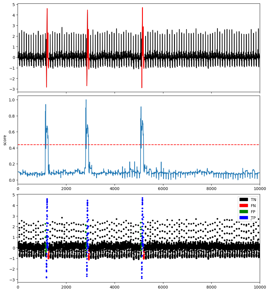
Histogram-based outlier detection (HBOS) [Goldstein et al. 2012] is an efficient unsupervised method. It assumes the feature independence and calculates the degree of outlyingness by building histograms. The methods is not dedicated for time series. Neverhteless, it can be used for point anomaly detection and subsequence as well, if we consider a subsequence as a vector.
- class TSB_UAD.models.hbos.HBOS(*args: Any, **kwargs: Any)
Histogram- based outlier detection (HBOS) implementation
- Parameters
n_bins (
int,optional (default=10)) – The number of bins.alpha (
float in (0,1),optional (default=0.1)) – The regularizer for preventing overflow.tol (
float in (0,1),optional (default=0.5)) – The parameter to decide the flexibility while dealing the samples falling outside the bins.contamination (
float in (0.,0.5),optional (default=0.1)) – The amount of contamination of the data set, i.e. the proportion of outliers in the data set. Used when fitting to define the threshold on the decision function.
- decision_scores_
The outlier scores of the training data. The higher, the more abnormal. Outliers tend to have higher scores. This value is available once the detector is fitted.
- Type
numpy arrayofshape (n_samples,)
- bin_edges_
The edges of the bins.
- Type
numpy arrayofshape (n_bins + 1,n_features )
- hist_
The density of each histogram.
- Type
numpy arrayofshape (n_bins,n_features)
- threshold_
The threshold is based on
contamination. It is then_samples * contaminationmost abnormal samples indecision_scores_. The threshold is calculated for generating binary outlier labels.- Type
- labels_
The binary labels of the training data. 0 stands for inliers and 1 for outliers/anomalies. It is generated by applying
threshold_ondecision_scores_.- Type
int,either 0or1
- decision_function(X)
Predict raw anomaly score of X using the fitted detector. The anomaly score of an input sample is computed based on different detector algorithms. For consistency, outliers are assigned with larger anomaly scores.
- Parameters
X (
numpy arrayofshape (n_samples,n_features)) – The training input samples. Sparse matrices are accepted only if they are supported by the base estimator.- Returns
anomaly_scores – The anomaly score of the input samples.
- Return type
numpy arrayofshape (n_samples,)
- fit(X, y=None)
Fit detector. y is ignored in unsupervised methods.
- Parameters
X (
numpy arrayofshape (n_samples,n_features)) – The input samples (time series length). n_features corresponds to the subsequence length.y (
Ignored) – Not used, present for API consistency by convention.
- Returns
self – Fitted estimator.
- Return type
import os
import numpy as np
import pandas as pd
from TSB_UAD.utils.visualisation import plotFig
from TSB_UAD.models.hbos import HBOS
from TSB_UAD.models.feature import Window
from TSB_UAD.utils.slidingWindows import find_length
from TSB_UAD.vus.metrics import get_metrics

#Read data
filepath = 'PATH_TO_TSB_UAD/ECG/MBA_ECG805_data.out'
df = pd.read_csv(filepath, header=None).dropna().to_numpy()
name = filepath.split('/')[-1]

data = df[:,0].astype(float)
label = df[:,1].astype(int)

#Pre-processing
slidingWindow = find_length(data)
X_data = Window(window = slidingWindow).convert(data).to_numpy()


#Run HBOS
modelName='PCA'
clf = HBOS()
clf.fit(X_data)
score = clf.decision_scores_

# Post-processing
score = MinMaxScaler(feature_range=(0,1)).fit_transform(score.reshape(-1,1)).ravel()
score = np.array([score[0]]*math.ceil((slidingWindow-1)/2) + list(score) + [score[-1]]*((slidingWindow-1)//2))


#Plot result
plotFig(data, label, score, slidingWindow, fileName=name, modelName=modelName)

#Print accuracy
results = get_metrics(score, label, metric="all", slidingWindow=slidingWindow)
for metric in results.keys():
    print(metric, ':', results[metric])
Example
References
[Goldstein et al. 2012] Goldstein, Markus and Andreas R. Dengel. “Histogram-based Outlier Score (HBOS): A fast Unsupervised Anomaly Detection Algorithm.” (2012).
One-Class Support Vector Machine (OCSVM)
One-Class Support Vector Machine (OCSVM) is a typical distribution-based example, which aims to separate the instances from an origin and maximize the distance from the hyperplane separation [Schölkopf et al. 1999] or spherical separation [Tax and Duin 2004]. The anomalies are identified with points of high decision score, i.e., far away from the separation hyper-plane. This method is a variant of the classical Support Vector Machine for classification tasks [Hearst et al. 1998].
The TSB-UAD implementation of OCSVM is a wrapper of Scikit-learn implementation of OneClassSVM.
- class TSB_UAD.models.ocsvm.OCSVM(*args: Any, **kwargs: Any)
Wrapper of scikit-learn one-class SVM Class with more functionalities.
- Parameters
kernel (
string, optional, default'rbf') – Specifies the kernel type to be used in the algorithm. It must be one of ‘linear’, ‘poly’, ‘rbf’, ‘sigmoid’, ‘precomputed’ or a callable. If none is given, ‘rbf’ will be used. If a callable is given it is used to precompute the kernel matrix.nu (
float, optional) – An upper bound on the fraction of training errors and a lower bound of the fraction of support vectors. Should be in the interval (0, 1]. By default 0.5 will be taken.degree (
int,optional (default=3)) – Degree of the polynomial kernel function (‘poly’). Ignored by all other kernels.gamma (
float, optional, default'auto') – Kernel coefficient for ‘rbf’, ‘poly’ and ‘sigmoid’. If gamma is ‘auto’ then 1/n_features will be used instead.coef0 (
float,optional (default=0.0)) – Independent term in kernel function. It is only significant in ‘poly’ and ‘sigmoid’.tol (
float, optional) – Tolerance for stopping criterion.shrinking (
bool, optional) – Whether to use the shrinking heuristic.cache_size (
float, optional) – Specify the size of the kernel cache (in MB).verbose (
bool, default:False) – Enable verbose output. Note that this setting takes advantage of a per-process runtime setting in libsvm that, if enabled, may not work properly in a multithreaded context.max_iter (
int,optional (default=-1)) – Hard limit on iterations within solver, or -1 for no limit.contamination (
float in (0.,0.5),optional (default=0.1)) – The amount of contamination of the data set, i.e. the proportion of outliers in the data set. Used when fitting to define the threshold on the decision function.
- decision_scores_
The outlier scores of the training data. The higher, the more abnormal. Outliers tend to have higher scores. This value is available once the detector is fitted.
- Type
numpy arrayofshape (n_samples,)
- support_
Indices of support vectors.
- Type
array-like,shape = [n_SV]
- support_vectors_
Support vectors.
- Type
array-like,shape = [nSV,n_features]
- dual_coef_
Coefficients of the support vectors in the decision function.
- Type
array,shape = [1,n_SV]
- coef_
Weights assigned to the features (coefficients in the primal problem). This is only available in the case of a linear kernel. coef_ is readonly property derived from dual_coef_ and support_vectors_
- Type
array,shape = [1,n_features]
- intercept_
Constant in the decision function.
- Type
array,shape = [1,]
- threshold_
The threshold is based on
contamination. It is then_samples * contaminationmost abnormal samples indecision_scores_. The threshold is calculated for generating binary outlier labels.- Type
- labels_
The binary labels of the training data. 0 stands for inliers and 1 for outliers/anomalies. It is generated by applying
threshold_ondecision_scores_.- Type
int,either 0or1
- decision_function(X)
Predict raw anomaly score of X using the fitted detector. The anomaly score of an input sample is computed based on different detector algorithms. For consistency, outliers are assigned with larger anomaly scores.
- Parameters
X (
numpy arrayofshape (n_samples,n_features)) – The training input samples. Sparse matrices are accepted only if they are supported by the base estimator.- Returns
anomaly_scores – The anomaly score of the input samples.
- Return type
numpy arrayofshape (n_samples,)
- fit(X_train, X_test, y=None, sample_weight=None, **params)
Fit detector. y is ignored in unsupervised methods.
- Parameters
X (
numpy arrayofshape (n_samples,n_features)) – The input samples.y (
Ignored) – Not used, present for API consistency by convention.sample_weight (
array-like,shape (n_samples,)) – Per-sample weights. Rescale C per sample. Higher weights force the classifier to put more emphasis on these points.
- Returns
self – Fitted estimator.
- Return type
Example
import os
import numpy as np
import pandas as pd
from TSB_UAD.utils.visualisation import plotFig
from TSB_UAD.models.ocsvm import OCSVM
from TSB_UAD.models.feature import Window
from TSB_UAD.utils.slidingWindows import find_length
from TSB_UAD.vus.metrics import get_metrics

#Read data
filepath = 'PATH_TO_TSB_UAD/ECG/MBA_ECG805_data.out'
df = pd.read_csv(filepath, header=None).dropna().to_numpy()
name = filepath.split('/')[-1]

data = df[:,0].astype(float)
label = df[:,1].astype(int)

#Pre-processing
slidingWindow = find_length(data)
data_train = data[:int(0.1*len(data))]
data_test = data

X_train = Window(window = slidingWindow).convert(data_train).to_numpy()
X_test = Window(window = slidingWindow).convert(data_test).to_numpy()

X_train_ = MinMaxScaler(feature_range=(0,1)).fit_transform(X_train.T).T
X_test_ = MinMaxScaler(feature_range=(0,1)).fit_transform(X_test.T).T


#Run OCSVM
modelName='OCSVM'
clf = OCSVM(nu=0.05)
clf.fit(X_train_, X_test_)
score = clf.decision_scores_

# Post-processing
score = np.array([score[0]]*math.ceil((slidingWindow-1)/2) + list(score) + [score[-1]]*((slidingWindow-1)//2))
score = MinMaxScaler(feature_range=(0,1)).fit_transform(score.reshape(-1,1)).ravel()

#Plot result
plotFig(data, label, score, slidingWindow, fileName=name, modelName=modelName)

#Print accuracy
results = get_metrics(score, label, metric="all", slidingWindow=slidingWindow)
for metric in results.keys():
    print(metric, ':', results[metric])
AUC_ROC : 0.9416967787322199
AUC_PR : 0.4592289027872978
Precision : 0.6402266288951841
Recall : 0.7458745874587459
F : 0.6890243902439025
Precision_at_k : 0.7458745874587459
Rprecision : 0.4007206588881263
Rrecall : 0.7967914438502675
RF : 0.5332568942659819
R_AUC_ROC : 0.9983442451461604
R_AUC_PR : 0.9119783238745204
VUS_ROC : 0.9905101824629529
VUS_PR : 0.8021253491270806
Affiliation_Precision : 0.9798093961448288
Affiliation_Recall : 0.9970749874410433
References
[Schölkopf et al. 1999] B. Sch ̈olkopf, R. C. Williamson, A. Smola, J. Shawe-Taylor, and J. Platt. 1999. Support vector method for novelty detection. NeurIPS, 12.
[Tax and Duin 2004] D. M. Tax and R. P. Duin. 2004. Support vector data description. Machine learning, 54(1): 45–66.
[Hearst et al. 1998] M. A. Hearst, S. T. Dumais, E. Osuna, J. Platt, and B. Scholkopf. July 1998. Support vector machines. IEEE Intelligent Systems and their Applications, 13(4): 18–28. ISSN 1094-7167. DOI: 10.1109/5254.708428