
Forecasting-based methods
Long Short-Term Memory Anomaly Detection (LSTM)
Long Short-Term Memory (LSTM) [Hochreiter and Schmidhuber 1997] network has been demonstrated to be particularly efficient in learning inner features for sub-sequences classification or time series forecasting. Such a model can also be used for anomaly detection purposes [Filonov et al. 2016, Malhotra et al. 2015]. The two latter papers’ principle is as follows: A stacked LSTM model is trained on normal parts of the data. The objective is to predict the following point or the subsequence using the previous ones. Consequently, the model will be trained to forecast a healthy state of the time series, and, therefore, will fail to forecast when it will encounter an anomaly.
The implementation of TSB-UAD corresponds to LSTM-AD [Malhotra et al. 2015].
- class TSB_UAD.models.lstm.lstm(slidingwindow=100, predict_time_steps=1, epochs=10, patience=10, verbose=0)
Implementation of LSTM-AD
- Parameters
- decision_scores_
The anomaly score. The higher, the more abnormal. Anomalies tend to have higher scores. This value is available once decision_function is called.
- Type
numpy arrayofshape (n_samples - subsequence_length,)
- decision_function(measure=None)
Derive the decision score based on the given distance measure
- fit(X_clean, X_dirty, ratio=0.15)
Fit detector.
- Parameters
X_clean (
numpy arrayofshape (n_samples,)) – The input training samples.X_dirty (
numpy arrayofshape (n_samples,)) – The input testing samples.ratio (
flaot,([0,1])) – The ratio for the train validation split
- Returns
self – Fitted estimator.
- Return type
Example
import os
import numpy as np
import pandas as pd
from TSB_UAD.utils.visualisation import plotFig
from TSB_UAD.models.distance import Fourier
from TSB_UAD.models.lstm import lstm
from TSB_UAD.models.feature import Window
from TSB_UAD.utils.slidingWindows import find_length
from TSB_UAD.vus.metrics import get_metrics
#Read data
filepath = 'PATH_TO_TSB_UAD/ECG/MBA_ECG805_data.out'
df = pd.read_csv(filepath, header=None).dropna().to_numpy()
name = filepath.split('/')[-1]
data = df[:,0].astype(float)
label = df[:,1].astype(int)
#Pre-processing
slidingWindow = find_length(data)
data_train = data[:int(0.1*len(data))]
data_test = data
#Run LSTM
modelName='LSTM'
clf = lstm(slidingwindow = slidingWindow, predict_time_steps=1, epochs = 50, patience = 5, verbose=0)
clf.fit(data_train, data_test)
measure = Fourier()
measure.detector = clf
measure.set_param()
clf.decision_function(measure=measure)
# Post-processing
score = MinMaxScaler(feature_range=(0,1)).fit_transform(score.reshape(-1,1)).ravel()
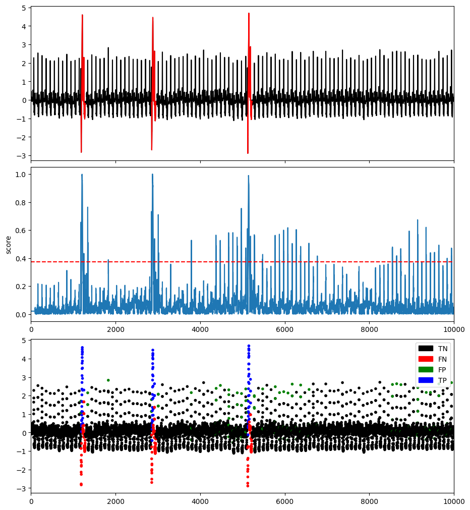
#Plot result
plotFig(data, label, score, slidingWindow, fileName=name, modelName=modelName)
#Print accuracy
results = get_metrics(score, label, metric="all", slidingWindow=slidingWindow)
for metric in results.keys():
print(metric, ':', results[metric])
AUC_ROC : 0.6831383664302287
AUC_PR : 0.120628447738072
Precision : 0.18439716312056736
Recall : 0.1716171617161716
F : 0.17777777777777776
Precision_at_k : 0.1716171617161716
Rprecision : 0.025
Rrecall : 0.3118637353931472
RF : 0.04628930078050358
R_AUC_ROC : 0.7300452172501921
R_AUC_PR : 0.14859987239776568
VUS_ROC : 0.7275909879072169
VUS_PR : 0.1426549169000135
Affiliation_Precision : 0.6036749472429264
Affiliation_Recall : 0.9836496679878174

References
[Hochreiter and Schmidhuber 1997] S. Hochreiter and J. Schmidhuber. Nov. 1997. Long short-term memory. Neural Comput., 9(8): 1735–1780.
[Filonov et al. 2016] P. Filonov, A. Lavrentyev, and A. Vorontsov. 2016. Multivariate industrial time series with cyber-attack simulation: Fault detection using an lstm-based predictive data model. arXiv preprint arXiv:1612.06676.
[Malhotra et al. 2015] P. Malhotra, L. Vig, G. Shroff, P. Agarwal, et al. 2015. Long short term memory networks for anomaly detection in time series. In Esann, volume 2015, p. 89.
Concolutional Neural Network-based Anomaly Detection (CNN)
This method, called DeepAnt [Munir et al. 2019], is a forecasting-based approach that build a non-linear relationship between current and previous time series points or subsequences (using convolutional Neural Network). The outliers are detected by the deviation between the predicted and actual values.
- class TSB_UAD.models.cnn.cnn(slidingwindow=100, predict_time_steps=1, epochs=10, patience=10, verbose=0)
Implementation of CNN
- Parameters
- decision_scores_
The anomaly score. The higher, the more abnormal. Anomalies tend to have higher scores. This value is available once decision_function is called.
- Type
numpy arrayofshape (n_samples - subsequence_length,)
- decision_function(measure=None)
Derive the decision score based on the given distance measure
- fit(X_clean, X_dirty, ratio=0.15)
Fit detector.
- Parameters
X_clean (
numpy arrayofshape (n_samples,)) – The input training samples.X_dirty (
numpy arrayofshape (n_samples,)) – The input testing samples.ratio (
flaot,([0,1])) – The ratio for the train validation split
- Returns
self – Fitted estimator.
- Return type
Example
import os
import numpy as np
import pandas as pd
from TSB_UAD.utils.visualisation import plotFig
from TSB_UAD.models.distance import Fourier
from TSB_UAD.models.cnn import cnn
from TSB_UAD.models.feature import Window
from TSB_UAD.utils.slidingWindows import find_length
from TSB_UAD.vus.metrics import get_metrics

#Read data
filepath = 'PATH_TO_TSB_UAD/ECG/MBA_ECG805_data.out'
df = pd.read_csv(filepath, header=None).dropna().to_numpy()
name = filepath.split('/')[-1]

data = df[:,0].astype(float)
label = df[:,1].astype(int)

#Pre-processing
slidingWindow = find_length(data)

data_train = data[:int(0.1*len(data))]
data_test = data


#Run CNN
clf = cnn(slidingwindow = slidingWindow, predict_time_steps=1, epochs = 100, patience = 5, verbose=0)
clf.fit(data_train, data_test)
measure = Fourier()
measure.detector = clf
measure.set_param()
clf.decision_function(measure=measure)
score = clf.decision_scores_

# Post-processing
score = MinMaxScaler(feature_range=(0,1)).fit_transform(score.reshape(-1,1)).ravel()
#Plot result
plotFig(data, label, score, slidingWindow, fileName=name, modelName=modelName)

#Print accuracy
results = get_metrics(score, label, metric="all", slidingWindow=slidingWindow)
for metric in results.keys():
    print(metric, ':', results[metric])
AUC_ROC : 0.8223519165363994
AUC_PR : 0.3990233632226723
Precision : 0.4337899543378995
Recall : 0.31353135313531355
F : 0.36398467432950193
Precision_at_k : 0.31353135313531355
Rprecision : 0.08823529411764706
Rrecall : 0.32537136066547834
RF : 0.13882386742945993
R_AUC_ROC : 0.8822285204143624
R_AUC_PR : 0.3932986259608648
VUS_ROC : 0.8811101069489891
VUS_PR : 0.4065135625548785
Affiliation_Precision : 0.9128891170124862
Affiliation_Recall : 0.9900155246934222
References
[Munir et al. 2019] M. Munir, S. A. Siddiqui, A. Dengel, and S. Ahmed. 2019. DeepAnT: A Deep Learning Approach for Unsupervised Anomaly Detection in Time Series. 7: 1991–2005. ISSN 2169-3536. DOI:10.1109/ACCESS.2018.2886457.