
Encoding-based methods
Principal Component Analysis-based Anomaly Detection (PCA)
The first encoding-based approach is to encode and represent the time series with its principal components. Principal Components Analysis (PCA) investigates the major components of the time series that contribute the most to the covariance structure. The anomaly score is measured by the sub-sequences distance from 0 along the principal components weighted by their eigenvalues. Please see [Aggarwal 2015] for mre details.
The TSB-UAD implementation of PCA is adapted from PyOD implementation [Zhao et al. 2019].
- class TSB_UAD.models.pca.PCA(*args: Any, **kwargs: Any)
PCA class modifed over from PYOD package
- Parameters
n_components (
int,float,Noneorstring) – Number of components to keep. if n_components is not set all components are kept. if n_components == ‘mle’ and svd_solver == ‘full’, Minka’s MLE is used to guess the dimension if0 < n_components < 1and svd_solver == ‘full’, select the number of components such that the amount of variance that needs to be explained is greater than the percentage specified by n_components n_components cannot be equal to n_features for svd_solver == ‘arpack’.n_selected_components (
int,optional (default=None)) – Number of selected principal components for calculating the outlier scores. It is not necessarily equal to the total number of the principal components. If not set, use all principal components.contamination (
float in (0.,0.5),optional (default=0.1)) – The amount of contamination of the data set, i.e. the proportion of outliers in the data set. Used when fitting to define the threshold on the decision function.copy (
bool (default True)) – If False, data passed to fit are overwritten and running fit(X).transform(X) will not yield the expected results, use fit_transform(X) instead.whiten (
bool,optional (default False)) – When True (False by default) the components_ vectors are multiplied by the square root of n_samples and then divided by the singular values to ensure uncorrelated outputs with unit component-wise variances. Whitening will remove some information from the transformed signal (the relative variance scales of the components) but can sometime improve the predictive accuracy of the downstream estimators by making their data respect some hard-wired assumptions.svd_solver (string
{'auto', 'full', 'arpack', 'randomized'}) –Singular Value Decompositon solver.
if auto, the solver is selected by a default policy based on X.shape and n_components. if the input data is larger than 500x500 and the number of components to extract is lower than 80% of the smallest dimension of the data, then the more efficient ‘randomized’ method is enabled. Otherwise the exact full SVD is computed and optionally truncated afterwards.
if full run exact full SVD calling the standard LAPACK solver via scipy.linalg.svd and select the components by postprocessing
if arpack run SVD truncated to n_components calling ARPACK solver via scipy.sparse.linalg.svds. It requires strictly 0 < n_components < X.shape[1]
if randomized, run randomized SVD by the method of Halko et al.
tol (
float >= 0,optional (default .0)) – Tolerance for singular values computed by svd_solver == ‘arpack’.iterated_power (
int >= 0, or'auto', (default'auto')) – Number of iterations for the power method computed by svd_solver == ‘randomized’.random_state (
int,RandomState instanceorNone,optional (default None)) – If int, random_state is the seed used by the random number generator; If RandomState instance, random_state is the random number generator; If None, the random number generator is the RandomState instance used by np.random. Used whensvd_solver== ‘arpack’ or ‘randomized’.weighted (
bool,optional (default=True)) – If True, the eigenvalues are used in score computation. The eigenvectors with small eigenvalues comes with more importance in outlier score calculation.standardization (
bool,optional (default=True)) – If True, perform standardization first to convert data to zero mean and unit variance. See http://scikit-learn.org/stable/auto_examples/preprocessing/plot_scaling_importance.html
- decision_scores_
The outlier scores of the training data. The higher, the more abnormal. Outliers tend to have higher scores. This value is available once the detector is fitted.
- Type
numpy arrayofshape (n_samples,)
- components_
Principal axes in feature space, representing the directions of maximum variance in the data. The components are sorted by
explained_variance_.- Type
array,shape (n_components,n_features)
- explained_variance_
The amount of variance explained by each of the selected components. Equal to n_components largest eigenvalues of the covariance matrix of X.
- Type
array,shape (n_components,)
- explained_variance_ratio_
Percentage of variance explained by each of the selected components. If
n_componentsis not set then all components are stored and the sum of explained variances is equal to 1.0.- Type
array,shape (n_components,)
- singular_values_
The singular values corresponding to each of the selected components. The singular values are equal to the 2-norms of the
n_componentsvariables in the lower-dimensional space.- Type
array,shape (n_components,)
- mean_
Per-feature empirical mean, estimated from the training set. Equal to X.mean(axis=0).
- Type
array,shape (n_features,)
- n_components_
The estimated number of components. When n_components is set to ‘mle’ or a number between 0 and 1 (with svd_solver == ‘full’) this number is estimated from input data. Otherwise it equals the parameter n_components, or n_features if n_components is None.
- Type
- noise_variance_
The estimated noise covariance following the Probabilistic PCA model from Tipping and Bishop 1999. See “Pattern Recognition and Machine Learning” by C. Bishop, 12.2.1 p. 574 or http://www.miketipping.com/papers/met-mppca.pdf. It is required to computed the estimated data covariance and score samples. Equal to the average of (min(n_features, n_samples) - n_components) smallest eigenvalues of the covariance matrix of X.
- Type
- threshold_
The threshold is based on
contamination. It is then_samples * contaminationmost abnormal samples indecision_scores_. The threshold is calculated for generating binary outlier labels.- Type
- labels_
The binary labels of the training data. 0 stands for inliers and 1 for outliers/anomalies. It is generated by applying
threshold_ondecision_scores_.- Type
int,either 0or1
- decision_function(X)
Predict raw anomaly score of X using the fitted detector. The anomaly score of an input sample is computed based on different detector algorithms. For consistency, outliers are assigned with larger anomaly scores.
- Parameters
X (
numpy arrayofshape (n_samples,n_features)) – The training input samples. Sparse matrices are accepted only if they are supported by the base estimator.- Returns
anomaly_scores – The anomaly score of the input samples.
- Return type
numpy arrayofshape (n_samples,)
- fit(X, y=None)
Fit detector. y is ignored in unsupervised methods.
- Parameters
X (
numpy arrayofshape (n_samples,n_features)) – The input samples (time series length). n_features corresponds to the subsequence length.y (
Ignored) – Not used, present for API consistency by convention.
- Returns
self – Fitted estimator.
- Return type
Example
import os
import numpy as np
import pandas as pd
from TSB_UAD.utils.visualisation import plotFig
from TSB_UAD.models.pca import PCA
from TSB_UAD.models.feature import Window
from TSB_UAD.utils.slidingWindows import find_length
from TSB_UAD.vus.metrics import get_metrics
#Read data
filepath = 'PATH_TO_TSB_UAD/ECG/MBA_ECG805_data.out'
df = pd.read_csv(filepath, header=None).dropna().to_numpy()
name = filepath.split('/')[-1]
data = df[:,0].astype(float)
label = df[:,1].astype(int)
#Pre-processing
slidingWindow = find_length(data)
X_data = Window(window = slidingWindow).convert(data).to_numpy()
#Run PCA
modelName='PCA'
clf = PCA()
clf.fit(X_data)
score = clf.decision_scores_
# Post-processing
score = MinMaxScaler(feature_range=(0,1)).fit_transform(score.reshape(-1,1)).ravel()
score = np.array([score[0]]*math.ceil((slidingWindow-1)/2) + list(score) + [score[-1]]*((slidingWindow-1)//2))
#Plot result
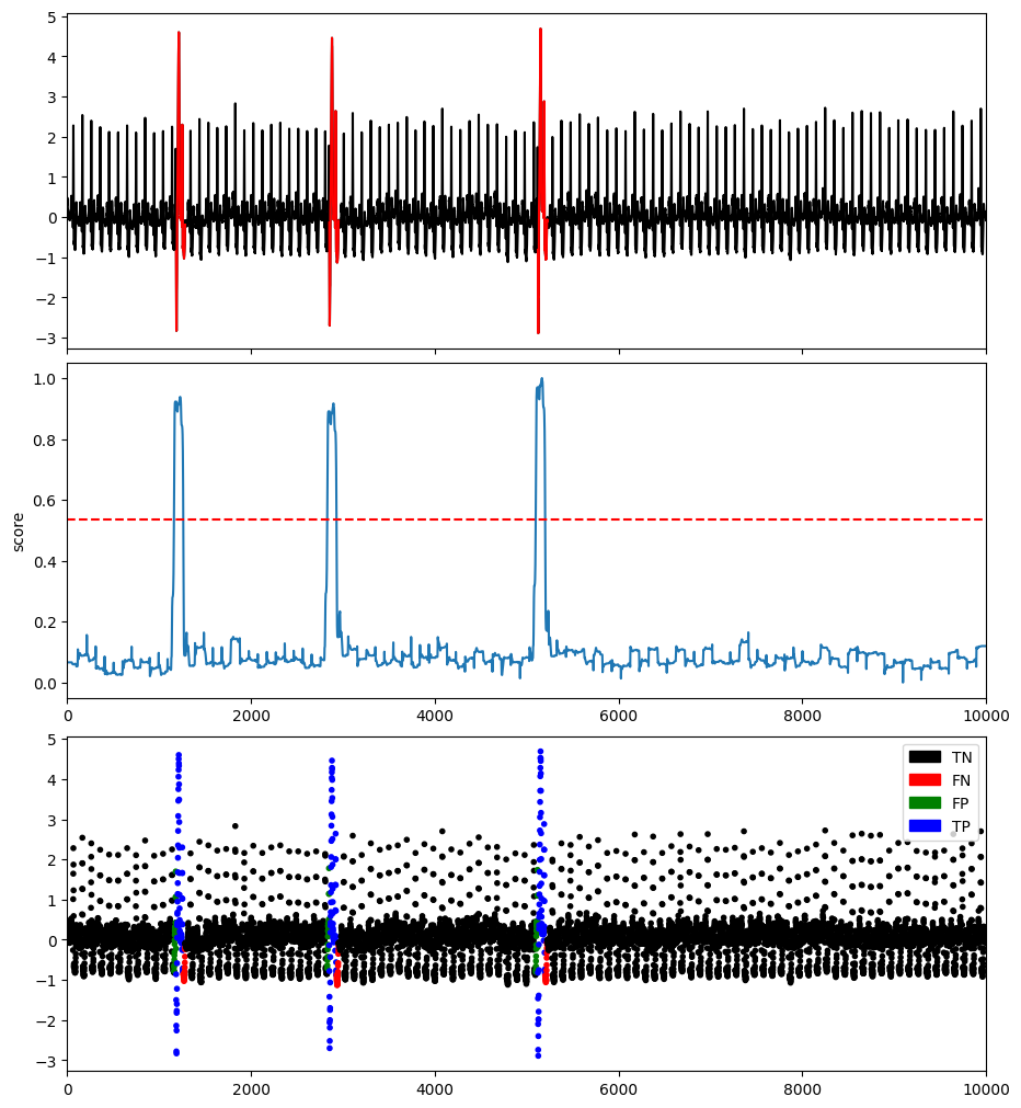
plotFig(data, label, score, slidingWindow, fileName=name, modelName=modelName)
#Print accuracy
results = get_metrics(score, label, metric="all", slidingWindow=slidingWindow)
for metric in results.keys():
print(metric, ':', results[metric])
AUC_ROC : 0.9831757023284056
AUC_PR : 0.7572161269856095
Precision : 0.7752442996742671
Recall : 0.7854785478547854
F : 0.7803278688524591
Precision_at_k : 0.7854785478547854
Rprecision : 0.77530626365804
Rrecall : 0.8284808873044168
RF : 0.8010120555743515
R_AUC_ROC : 0.9994595750446229
R_AUC_PR : 0.9836739288859631
VUS_ROC : 0.997118940672939
VUS_PR : 0.9475589866373976
Affiliation_Precision : 0.9890337001400605
Affiliation_Recall : 0.9982808225194953
References
[Aggarwal 2015] Charu C Aggarwal. Outlier analysis. In Data mining, 75–79. Springer, 2015.
[Zhao et al. 2019] Zhao, Yue, Zain Nasrullah and Zheng Li. PyOD: A Python Toolbox for Scalable Outlier Detection. J. Mach. Learn. Res. 20,2019.
Polynomial Approximation (POLY)
POLY is a encoding-based anoamly detection methods that aims to detect pointwise anomalies using polynomial approximation [Li et al. 2007]. A polynomial of certain degree and window size is fitted to the given time series dataset. A GARCH [Bollerslev 1986] method is ran on the difference betweeen the approximation and the true value of the dataset to estimate the volatitilies of each point. A score is derived on each point based on the estimated volatitilies and residual to measure the normality of each point. An alternative method that only considers absolute difference is also used.
- class TSB_UAD.models.poly.POLY(*args: Any, **kwargs: Any)
Polynomial Anomaly Detector with GARCH method and raw error method
- Parameters
Power (
int,optional (default=1)) – The power of polynomial fitted to the dataneighborhood (
int,optional (default=max (100,10*window size))) – The number of samples to fit for one subsequence. Since the timeseries may vary, to caculate the score for the subsequnece (a, a+k) of samples k, we only fit the polynomal on its neighborhood.window (
int,optional (default = 20)) – The length of the window to detect the given anomoliescontamination (
float in (0.,0.55),optional (default=0.1)) – The amount of contamination of the data set, i.e. the proportion of outliers in the data set. Used when fitting to define the threshold on the decision function.
- decision_scores_
The outlier scores of the training data. The higher, the more abnormal. Outliers tend to have higher scores. This value is available once the detector is fitted.
- Type
numpy arrayofshape (n_samples,)
- estimators_
The collection of fitted sub-estimators.
- Type
dictionaryofcoefficients at each polynomial
- threshold_
The threshold is based on
contamination. It is then_samples * contaminationmost abnormal samples indecision_scores_. The threshold is calculated for generating binary outlier labels.- Type
- labels_
The binary labels of the training data. 0 stands for inliers and 1 for outliers/anomalies. It is generated by applying
threshold_ondecision_scores_.- Type
int,either 0or1
- decision_function(X=False, measure=None)
Derive the decision score based on the given distance measure
- fit(X, y=None)
Fit detector. y is ignored in unsupervised methods.
- Parameters
X (
numpy arrayofshape (n_samples,)) – The input samples.y (
Ignored) – Not used, present for API consistency by convention.
- Returns
self – Fitted estimator.
- Return type
- predict_proba(X, method='linear', measure=None)
Predict the probability of a sample being outlier. Two approaches are possible:
simply use Min-max conversion to linearly transform the outlier scores into the range of [0,1]. The model must be fitted first.
use unifying scores.
- Parameters
X (
numpy arrayofshape (n_samples,n_features)) – The input samples.method (
str, optional, default'linear') – probability conversion method. It must be one of ‘linear’ or ‘unify’.
- Returns
outlier_probability – For each observation, tells whether or not it should be considered as an outlier according to the fitted model. Return the outlier probability, ranging in [0,1].
- Return type
numpy arrayofshape (n_samples,)
Example
import os
import numpy as np
import pandas as pd
from TSB_UAD.utils.visualisation import plotFig
from TSB_UAD.models.distance import Fourier
from TSB_UAD.models.poly import POLY
from TSB_UAD.models.feature import Window
from TSB_UAD.utils.slidingWindows import find_length
from TSB_UAD.vus.metrics import get_metrics

#Read data
filepath = 'PATH_TO_TSB_UAD/ECG/MBA_ECG805_data.out'
df = pd.read_csv(filepath, header=None).dropna().to_numpy()
name = filepath.split('/')[-1]

data = df[:,0].astype(float)
label = df[:,1].astype(int)

#Pre-processing
slidingWindow = find_length(data)


#Run POLY
modelName='POLY'
clf = POLY(power=3, window = slidingWindow)
clf.fit(data)
measure = Fourier()
measure.detector = clf
measure.set_param()
clf.decision_function(measure=measure)
score = clf.decision_scores_

# Post-processing
score = MinMaxScaler(feature_range=(0,1)).fit_transform(score.reshape(-1,1)).ravel()

#Plot result
plotFig(data, label, score, slidingWindow, fileName=name, modelName=modelName)

#Print accuracy
results = get_metrics(score, label, metric="all", slidingWindow=slidingWindow)
for metric in results.keys():
    print(metric, ':', results[metric])
AUC_ROC : 0.9958617394172128
AUC_PR : 0.8837102941063337
Precision : 0.8686868686868687
Recall : 0.8514851485148515
F : 0.86
Precision_at_k : 0.8514851485148515
Rprecision : 0.8686868686868686
Rrecall : 0.8821944939591999
RF : 0.875388577295774
R_AUC_ROC : 0.9966496859473177
R_AUC_PR : 0.9632279391916059
VUS_ROC : 0.9939772090687404
VUS_PR : 0.9465631009222253
Affiliation_Precision : 0.9810555530560522
Affiliation_Recall : 0.9999934905686477

References
[Li et al. 2007] Z. Li, H. Ma, and Y. Mei. 2007. A unifying method for outlier and change detection from data streams based on local polynomial fitting. In Z.-H. Zhou, H. Li, and Q. Yang, eds., Advances in Knowledge Discovery and Data Mining, pp. 150–161. Springer Berlin Heidelberg, Berlin, Heidelberg. ISBN 978-3-540-71701-0.
[Bollerslev 1986] Tim Bollerslev, Generalized autoregressive conditional heteroskedasticity, Journal of Econometrics, Volume 31, Issue 3, 1986, ISSN 0304-4076.